The Running Ultraviolet Spectrum of Galaxies
1. Introduction
Some nerds have been drawing things with their GPS watches/run trackers for
years. Typical 'GPS doodles' being Father Christmas, a hummingbird, and
(obviously) a massive schlong. In astronomy, everyone knows outreach with
imaging data is much easier than with spectra; it’s visualizable and people get it.
But there is also a (much hated, i hope) old saying
that goes something like 'you can do astronomy with imaging, but for
astrophysics you need spectra'. I regard myself as a physicist that has fallen
into observational astronomy. I also regard myself as a runner -- a crappy
runner, for sure, but I run a
lot. A few weeks ago, when looking at the pace of
a recent run in Strava (a figure of pace [=inverse speed] vs. distance along the
course) i pareidolia’d a noisy continuum (steady pace) with an
emission line (where I did some fast bits). This
triggered an idea that wouldn't go away: could I use similar techniques to recreate a convincing spectrum?
2. Real versus frequency space
More common 'GPS art' is easy in one way: walk, run, cycle, skateboard;
all that matters is the route. Nobody even looks at the pace after seeing the
hummingbird, and it really doesn't matter if you stop to orientate or for
coffee. My case is the reverse: the
course is irrelevant but timing, as they say, is everything. Depending upon the
object we are going to draw, we will need to control the pace -- or really the
pace contrast -- precisely.
3. Object selection
So what should I draw? I blackbody is probably too easy -- just accelerate
and decelerate. It’s also too unrealistic and unidentifiable. The same goes
for any other featureless spectrum like a blazar, and a very hot star (at least
in the optical) would just be an inverted progression run with a few small dips
for Balmer absorption. In contrast, all the silly features in cold stars would
make it a nightmare to run. Planetary nebulae would be cool, but with high
equivalent width emission lines it would need both lightning speed to get
the lines AND some veeeerrrry slow traipsing for the continuum. Broad-line
quasars would be possible -- at least then you have some time to accelerate, so
that’s an option. But I conclude that for my first attempt I should not diverge
too much from my field, so let’s try the UV spectrum
of a star-forming galaxy? It's got some discontinuities, some absorption lines
(absorption is easier than emission...), and a rather
interesting complicated
feature at 1216 Å (restframe).
4. Feature identification
I want some things that make it easy-to-identify, and some things to make it
cool. I decide to target a wavelength range from just shortwards of the Lyman
edge, so I can make a Lyman continuum emitter, and also cover significant
continuum redwards of Ly-alpha would be good to show some characteristic and
identifiable features in the spectrum, like high oscillator strength ISM
absorption lines (the resonance lines of metals), but the weaker lines and
stellar features will probably be lost in the noise (GPS is far from infinitely
precise; Sections 5 and 6).

Figure 1. The average spectrum of Lyman break galaxies at redshift around 3
(Shapley et al 2003, ApJ, 588, 65).
Basically it should look a bit like Figure 1, which is an average spectrum of
a distant galaxy (Shapley et al 2003), and I elect to include the following
features.
4.1. Included features (continuous)
- Lyman Continuum [880-912Å]. Pace = 12 mins/km
- Lyman edge to LyB (let’s include an IGM, characteristic of z~3)
[912-1025Å]. Pace = 10 mins/km
- LyB to LyA (somewhat less absorption) [1025-1216 Å]. Pace = 8 mins/km
- Remaining Balmer continuum to the edge of the ‘spectrograph’
[1216-1500Å]. Pace = 6 mins/km
4.2. Included features (discrete)
- 1190Å - Si II absorption line
- 1193Å - Si II absorption line
- 1216Å - Ly-alpha (let’s try a P Cygni)
- 1260Å - Si II absorption line
- 1302Å - O I absorption line
- 1304Å - Si II absorption line
- 1334Å - C II absorption line
So clearly the continuum is going to be a slow start, accelerating at the
discontinuities. Then for the absorption lines we will will have to slow to
zero (the lines are often black), wait for a GPS tick, and go back to the
previous pace. For Ly-alpha, which we will do as P Cygni we will have to go all
out for a few seconds to get the EW as high as possible, and then return to a
new pace to get the new continuum level. This could be hard.
5. The dispersion solution
Pace charts in Strava are displayed with distance on the x-axis. In Garmin
Connect they are displayed with time. Distance is much easier, as I can just
mark up features on the ground in chalk. Next we need a scaling between Å
in wavelength and m on the ground: too short and the thing will be too hard to
run, and the features undersampled/unresolved; too long and... I'll be running
for too long, and this will probably take a few tries… If I let 1 Å
corresponds to 2 m, I need to run 1240 m for the above example. In cartography
this would be a scale of 1:20,000,000,000; in observational astronomy it would
be a dispersion solution of 2×10¹⁰ Å/m [kind of taking
out the size of pixel].
I find a place without too much tree coverage and away from buildings for
maximum GPS performance, and mark out the relevant points on the tarmac using
my son's chalk (Figure 2).
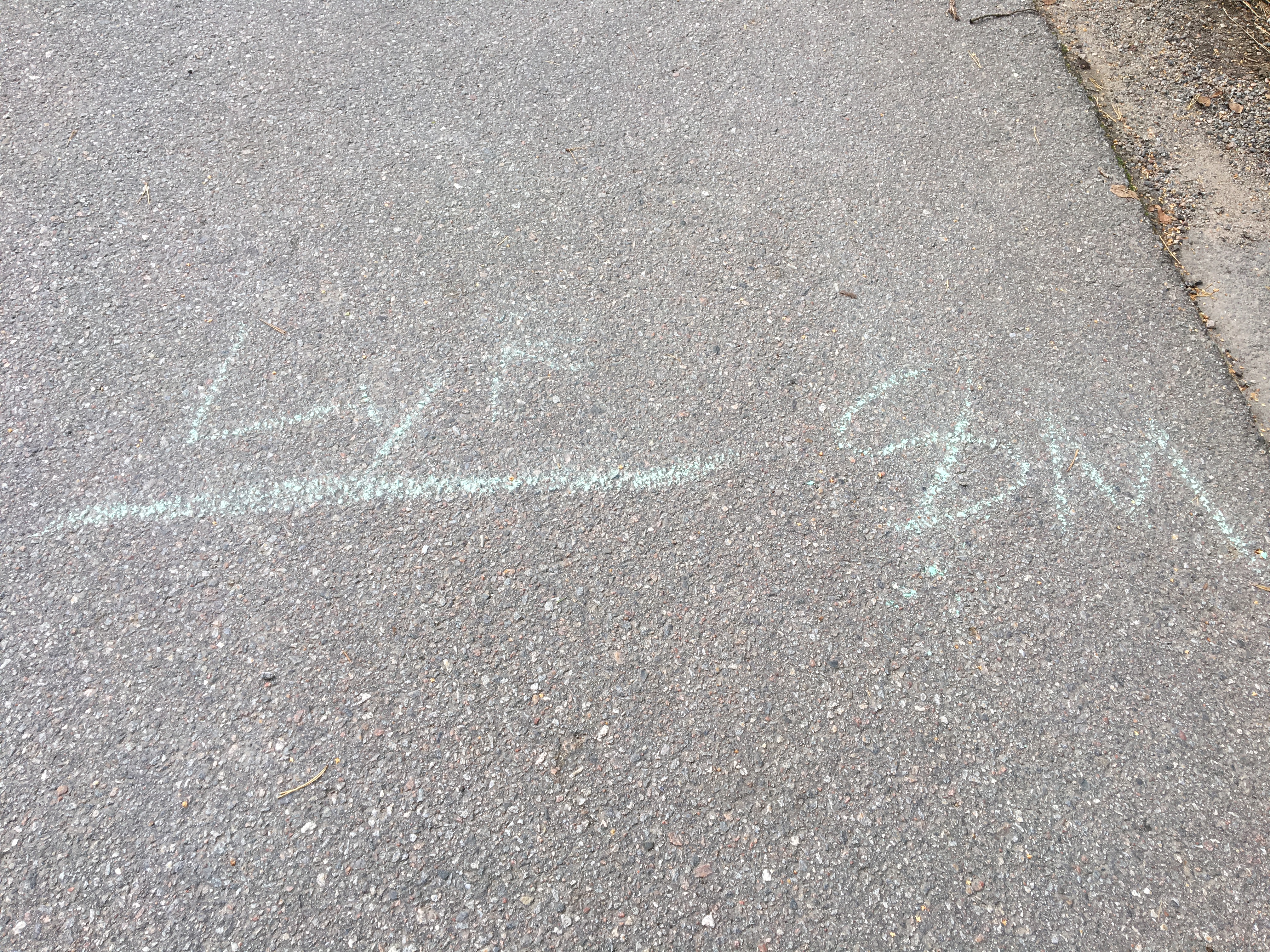
Figure 2. The transition at Ly-beta; new pace of 8 min/km. Didn't come out
very well, but good enough for running.
6. Sampling and precision -- the systematic SNR limit of the hardware.
The signal-to-noise ratio of the 'spectrum' will be set by the GPS precision.
I have a Garmin Forerunner 935 (Figure 3), which i have been happy with for pace
over a km and averaged over scales down to a few tens of m. Is it good enough
for this?
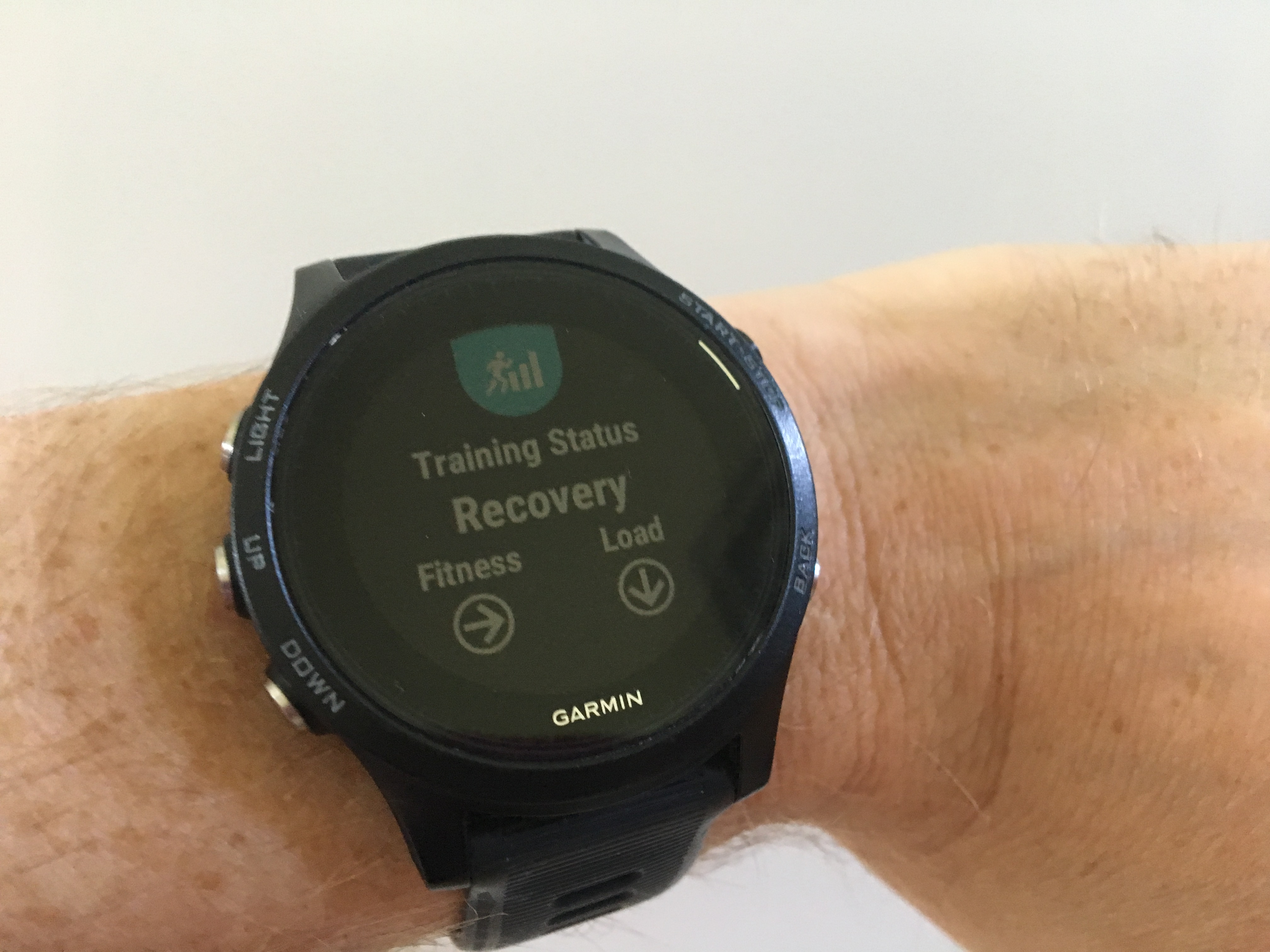
Figure 3. The Garmin Forerunner 935, telling me I am slacking off.
The Forerunner 935 supports GPS in combination with the Russian system
(GLONASS) and EU system (Galileo). I read a few blogs and learn that GLONASS is
fully operational while Galileo is not quite; however Galileo still has more
active satellites, and Garmin have also been prioritizing work on Galileo. I opt
for GPS+Galileo.
GPS sampling is time-based: the sampling rate (read: pixel size in Å (m))
will then be different depending upon how fast I run. I can make my watch tick
on 'Smart' mode (presumably varying with mode/speed) and Once-Per-Second.
As some of this (particularly LyC and absorption lines) will be done very
slowly, I go for once-per-second. At a pace of 6 min/km, 1 km takes 360 sec, so
it should tick every 2.77 m. Probably there is will be some smoothing in the
representation. I guess I have to pause for a few sec -- let’s say 3 -- to make
a black absorption line.
7. Execution
I go out and run the track. It’s really hard. Walking slow (LyC) is hard.
Walking 10 min/km is easy. Not speeding up when I see a transition coming is
hard. Running at 8 min/km is really hard. Stopping instantaneously is really
hard -- it’s very natural to slow down gradually, but that makes the absorption
lines too broad. Trusting that I got the lines in the correct place is
difficult. Also people think I look like a plum when I run and stop abbruptly on a chalk
line.
I run a few tries and go home.
8. Results
I load the data into both Strava and Garmin connect but these apps are so…
not orientated for UV spectroscopists that they don’t capture the essence. By
which I mean they oversmooth the data and don’t give me control over the axis
limits.. (Figure 4.)
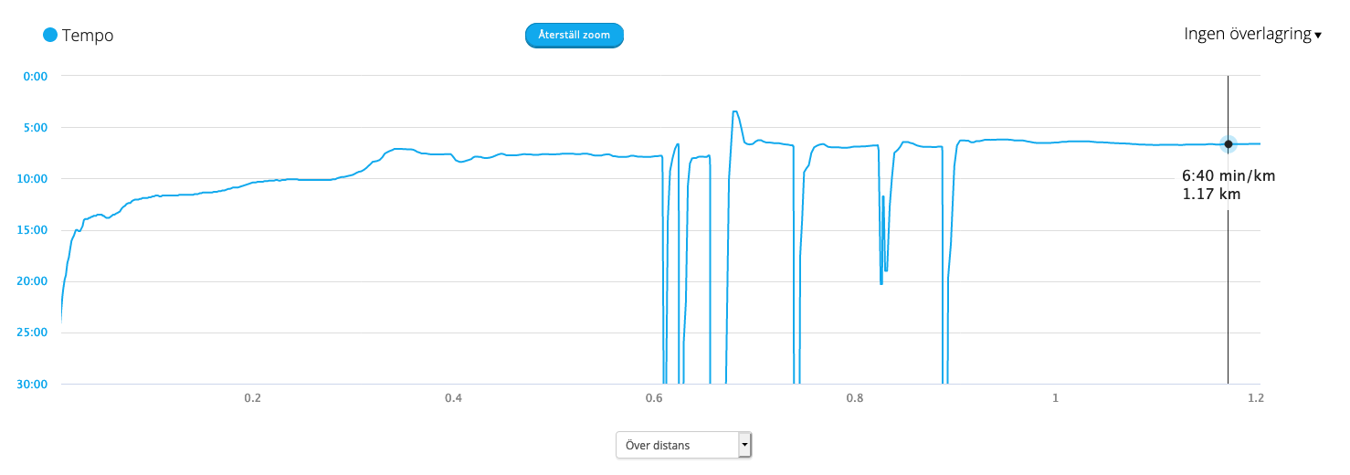
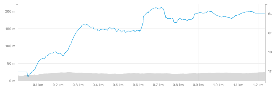
Figure 4. The spectra of run number 2, as displayed by Garmin (upper)
and Strava (lower).
Features are visible, but but the tools used by runners are clearly not
appropriate for this. Garmin's just looks terribly scaled, but you can see the
LyA, the break at LyB, and the absorption lines. Strava's looks a slitless
spectrograph, and we see broad features only. Damnit.. we can do better than this.
I download the GPX files and crack them open by hand and plot them using
python. It's easier than I thought to parse the XML, because obviously somebody
has already done this in python. There is a nice package called gpxpy that takes care of the
reading the GPX, and if you grab constants.R_earth from astropy then the rest is
easy. I smooth the data with a 1 second Gaussian kernel (3 m at 6 min/km).
Results, both uncalibrated data (in m) and calibrated (applying the
dispersion solution above), are shown in Figure 5. (Somehow these apps also
report instantaneous power output which has the same dimension as luminosity, so
I'm going to claim that the y-axis is already calibrated.)
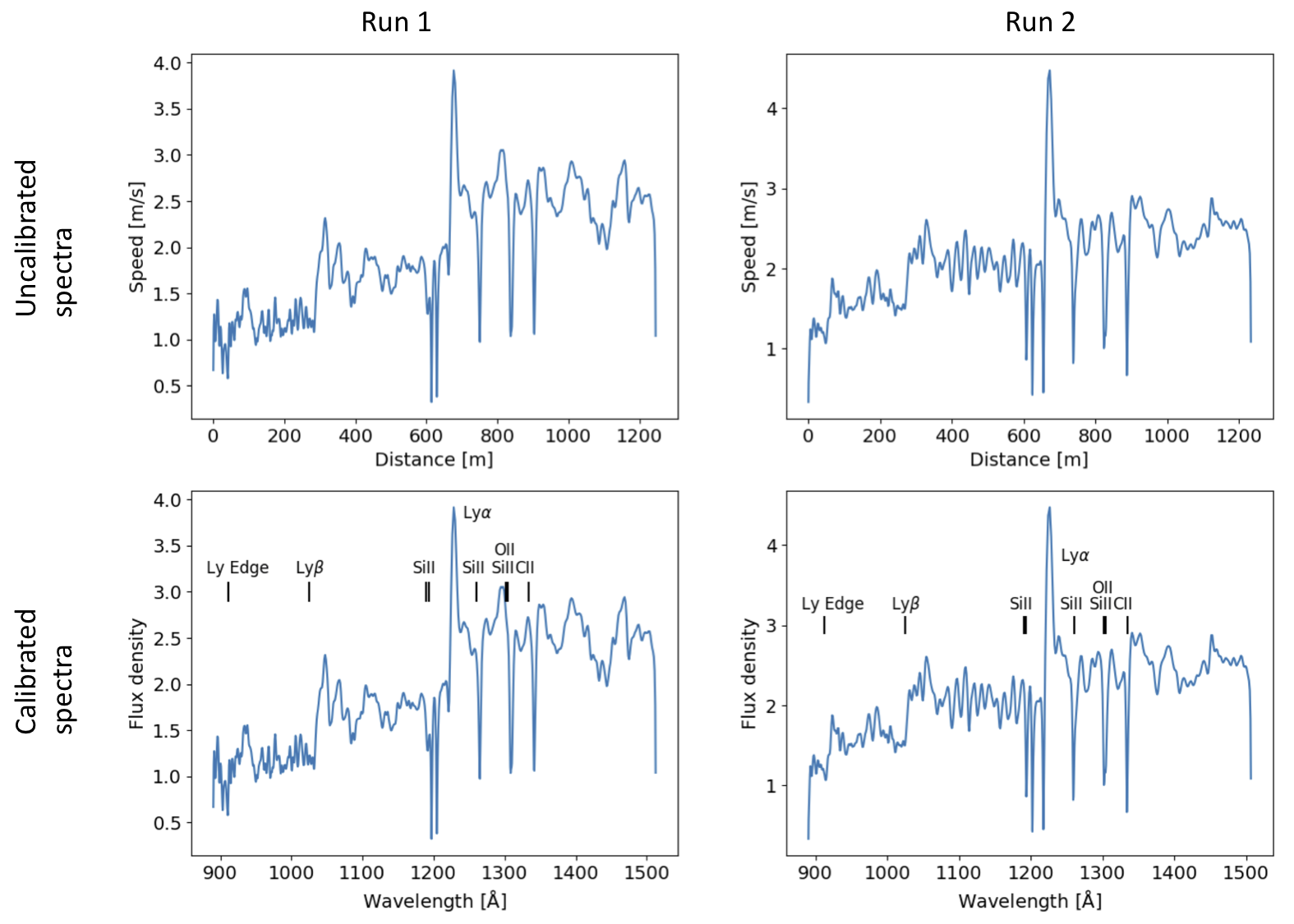
Figure 5. Uncalibrated (upper) and calibrated (lower) spectra of
star-forming galaxies, with main features identified.
Run 1 is shown to the left, and run 2 to the right.
This is much better than I thought -- It looks like IUE data! Run 2 gets the
absorption lines better (at least more uniform), but Run 1 seems to get the
breaks looking a bit more realistic. Low amplitude breaks from the IGM are visible at Ly-alpha and
Ly-beta (especially in run 1), but there is more LyC emission than I expected
(it's hard to walk at 15-18 min/km!). Resonance absorption lines are also
clear, especially in Run 2. I am very pleased with the Ly-alpha line: its P
Cygni shape is clear (especially in run 2) and the asymmetry on the red side is
also very clear. The equivalent widht is higher than I expected: that burst of
speed was apparently good enough (I guess I'm used only to looking at
over-smoothed data in Garmin), and I come out of it to a higher continuum level
than at shorter wavelengths.
9. Future perspectives and lessons learned
There are as many wavelength regions as you like to experiment with: I
haven’t played with optical through radio on the redder side. Going bluer,
perhaps the X-ray would be cool? You could put the x-axis in frequency, and the
y-axis in f-lambda, f-nu, or nu.f-nu.
And of course you don’t have to put wavel./frequency/energy on the x-axis,
and you could do time series stuff. I dunno. Pulsars, supernova light curves,
transiting exoplanets, whatever you like.
I have learned that I can produce an IUE-quality spectrum of a galaxy in
about 1-hour, which to order-of-magnitude is the same as the exposure time.
That’s enough for me.
Before anybody says I can enhance the SNR by doing it 100 times and stacking…
no.
|